Context

VLOOKUP is an Excel formula which looks up to the right to find a value.

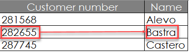
For instance, if you want to know which customer is #282655, VLOOKUP can help you for this: the formula will return “Bastra”.

But, what if you want to find the customer number of Castero? In this case, VLOOKUP will not help you. Indeed, as we said before, the formula only looks to the right, but in our example, the Customer numbers are in the left column.

I will show you three methods to solve this problem:

• Method A – Manual
• Method B – Nested formula (which works on every Excel’s versions)
• Method C – New era

Method A – Manual

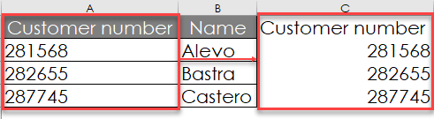
In this method, we will simply copy data from column A and paste them in column C. The result column (customer number) will be displayed to the right of the column with the desired value (name):

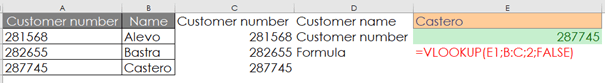
We are now able to perform the VLOOKUP, but the table array will be column B and C:

This method is easy, but not productive at all. Indeed, suppose that you have tons of data. Or that the data in column A are from an external source.

Method B – Nested formula

The advantage of this method is that it is working properly on every Excel’s versions (including the old versions). You can then share your file with everybody, it does not matter which Excel’s versions they have.

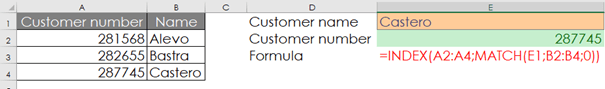
This method is using two formulas: INDEX (Uses an index to choose a value from a reference or array) and MATCH (Looks up values in a reference or array).

We will have:

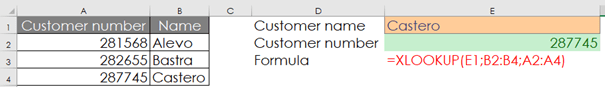
Method C – XLOOKUP

With Microsoft365, the firm from Redmond brought a gift for millions of Excel’s users: the VLOOKUP which looks to the left – XLOOKUP.

The structure of the formula is quite similar to the VLOOKUP, except that we must split the lookup array and the return array.

So, we will have:

---

You can download the file used as example here: